Basic Vector Processing & Analysis

This workbook is designed to introduce you with processing algorithms for working with vectors in QGIS.

By the end of the workbook, you should know: how to merge, split, and reproject vectors; create buffers, clips, intersections, etc; create grids and generate random points; create a simple model; and convert a raster to a vector.

Since this is a beginner workbook, no previous knowledge of GIS or QGIS is required.

Other learning resources

Official QGIS Documentation (QGIS 3.10)

Official QGIS Documentation (latest, QGIS 3.16)

BNHR blog

BNHR Facebook & Twitter & YouTube

Free and Open Source GIS Ramblings by Anita Graser

Klas Karlsson’s Youtube channel

QGIS User Group Philippines Facebook Page

Geographic Information Science Philippines Facebook Page

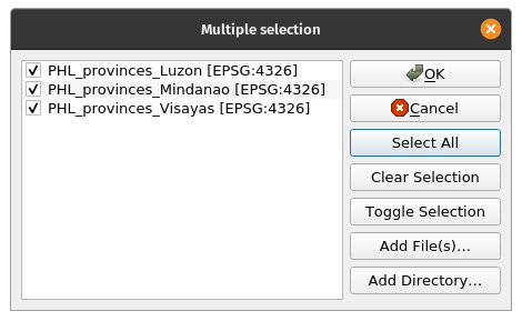
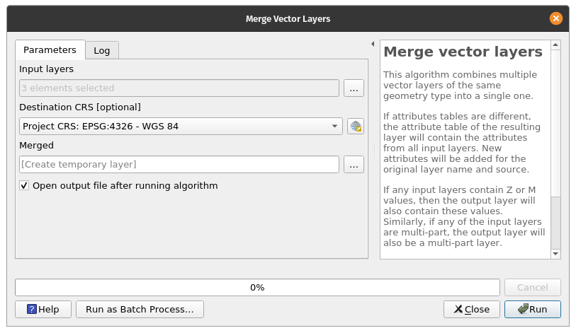
There are a variety of algorithms for working with vectors that can be found in QGIS’s built-in Processing provider. Aside from the core QGIS processing algorithms, QGIS also has access to algorithms provided by other processing providers such as applications like GRASS, SAGA, Orfeo Toolbox and processing plugins such as Whitebox Tools. QGIS algorithms can also be extended through the use of Python and R.

Merging vectors

Merging vectors is a common vector operation that combines several vector layers into one vector layer. This is useful when you want to create a larger dataset from multiple smaller datasets.

The Merge vector layers algorithm of QGIS combines multiple vector layers of the same geometry type into a single one. If attributes tables are different, the attribute table of the resulting layer will contain the attributes from all input layers. New attributes will be added for the original layer name and source.

Exercise 1: Merge the Luzon, Visayas, and Mindanao polygon layers to create a single Philippines polygon layer

1. Open the Merge vector layers by searching in the Locator Bar (CTRL + K) or via Vector -> Data Management -> Merge vector layers in the Menu bar.
2. Click on  on the Input layers and select the PHL_provinces_Luzon, PHL_provinces_Visayas, and PHL_provinces_MIndanao layers. If you already loaded the aforementioned layers in QGIS, you may select them directly in the selection window that appears. If not, you can add them by using the  or  buttons.
3. Set EPSG:4326 as the Destination CRS and store the result as a temporary layer.

4. Click Run.
5. You should see a layer named Merged added to the Layer panel. Rename this layer to PHL_provinces.

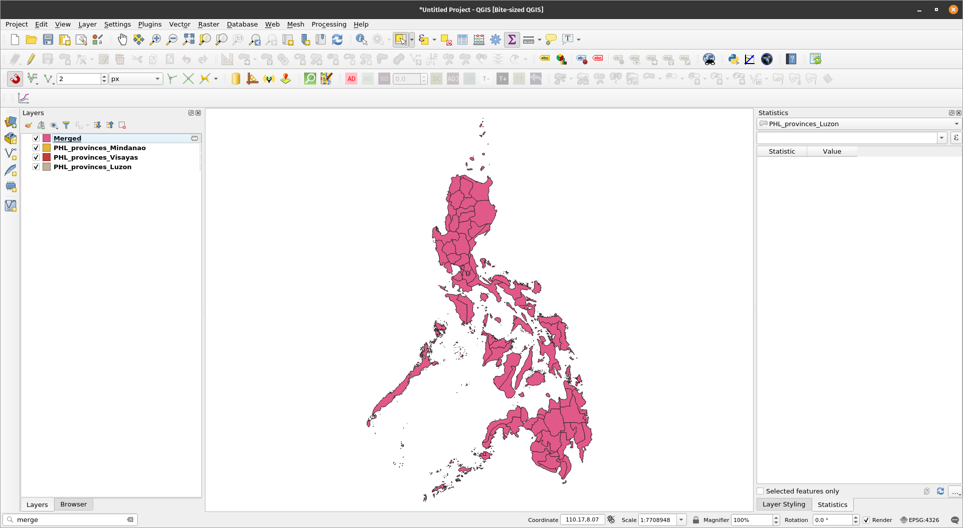
If you open the attribute table of this layer, it should have the same attributes as the other 3 layers. Notice also that this layer is a layer in memory or temporary layer. By default, the outputs of processing algorithms are temporary layers.

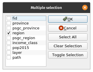
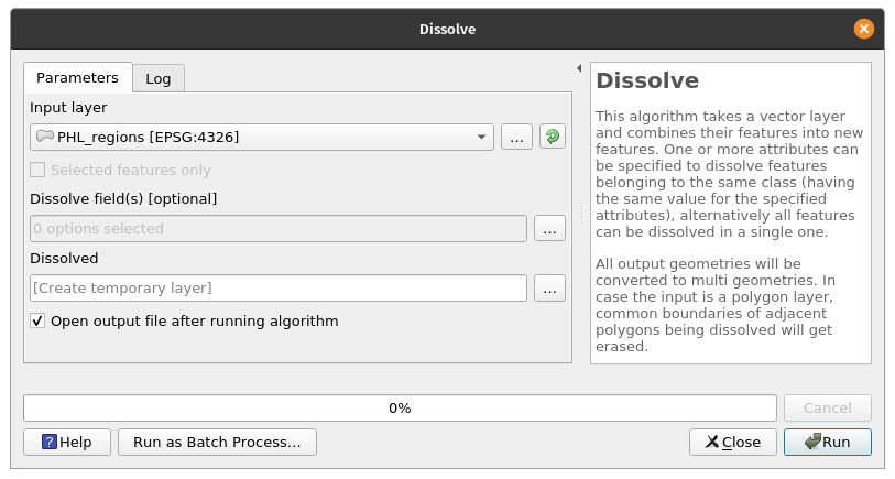
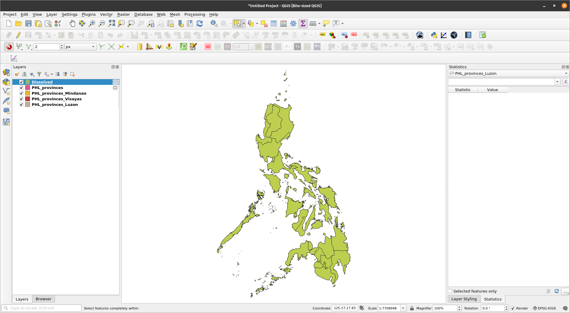
Dissolving vectors

The act of dissolving layers involves merging or combining features (geometries) based on their attributes.

The Dissolve algorithm in QGIS Processing takes a vector layer and combines their features into new features. One or more attributes can be specified to dissolve features belonging to the same class (having the same value for the specified attributes), alternatively all features can be dissolved in a single one.

All output geometries will be converted to multi geometries. In case the input is a polygon layer, common boundaries of adjacent polygons being dissolved will get erased.

Exercise 2: Dissolving the merged provincial polygon layer to create a regional polygon layer

For this exercise, we would like to create a regional polygon layer by dissolving the PHL_provinces layer based on its region or psgc_region attributes.

1. Open the Dissolve algorithm from the Locator Bar or via Vector -> Geoprocessing tools -> Dissolve in the Menu Bar. Notice that if you type Dissolve in the Locator Bar, more than one algorithm might appear -- Dissolve using GDAL, Dissolve using QGIS Processing, and v.dissolve if you have GRASS connected to QGIS. For this exercise, let’s use the Dissolve using QGIS Processing (usually the second in the list).
2. Click on  on the Dissolve fields option and select region.
3. Click Run.
4. You should see a layer named Dissolved added to the Layer panel. Rename this layer to PHL_regions.

If you open the attribute table of the PHL_regions layer, you might notice that there are still province and psgc_province attributes that don’t provide useful information (i.e. the features now correspond to regions and not provinces). You may delete or remove these attributes.

At this point, you may want to save your work as a project (CTRL + S) and use the Memory Layer Saver plugin to make your layers in memory persistent or export your PHL_provinces and PHL_regions provinces as vector files (e.g. as geopackage or geojson).

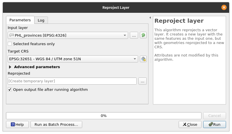
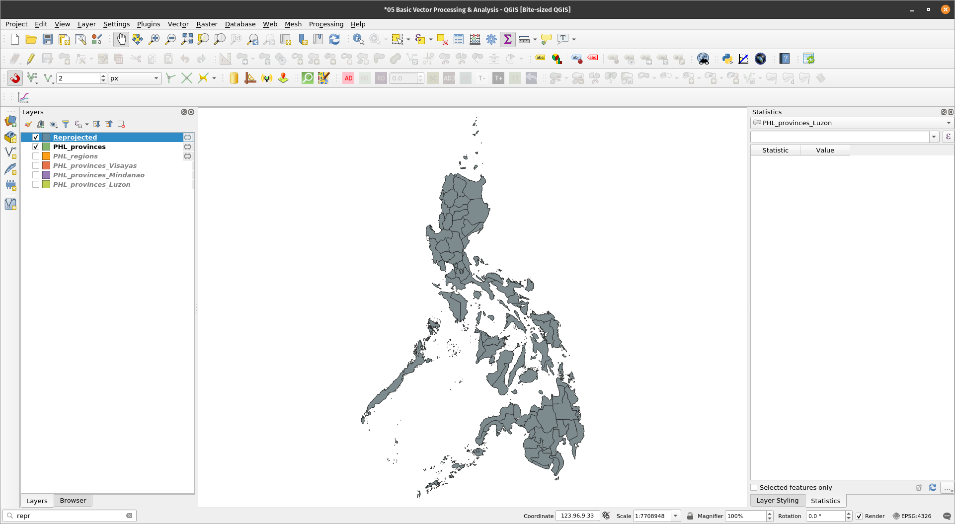
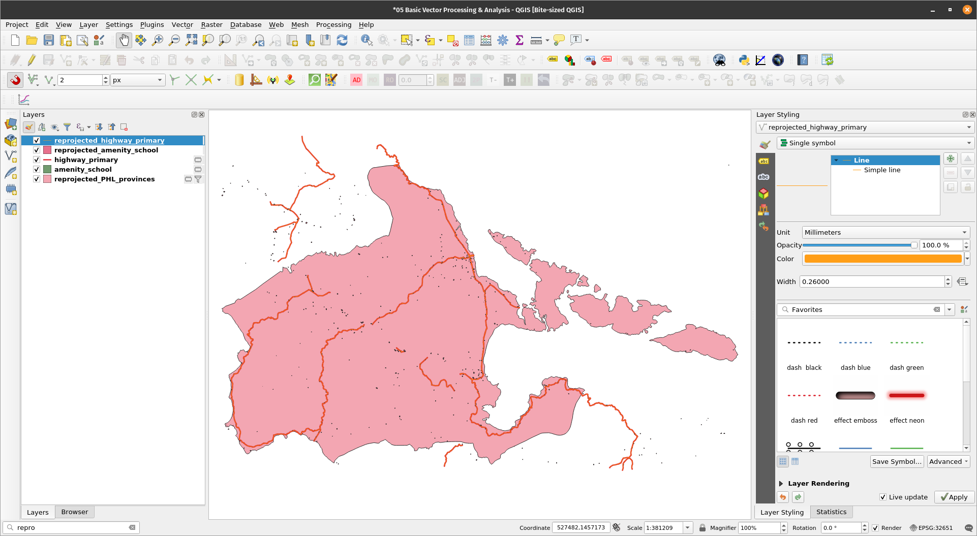
Reprojecting vectors

There are several ways to reproject vectors in QGIS. The simplest is by exporting the layer and setting the new CRS there. Another way is by using the Reproject algorithm.

Exercise 3: Reprojecting a vector from one CRS to another

1. Open the Reproject Layer algorithm by searching in the Locator Bar or via Vector -> Data Management Tools -> Reproject Layer in the Menu bar.

NOTE: If you use the Locator Bar, be sure to select the option under Processing Algorithms instead of Edit Selected Features.   

1. Input layer: PHL_provinces
2. Target CRS: EPSG: 32651

2. Click Run.
3. You should see a layer named Reprojected added to the Layer panel. Rename this layer to reprojected_PHL_provinces.

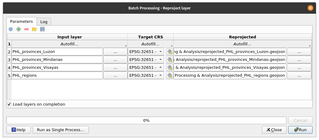
BONUS: The ability to perform batch processing is exposed for most processing algorithms. This option can normally be found in the lower left corner of a processing algorithm window.

By clicking , we can run a processing algorithm for several inputs. The Batch Process window will allow users to add parameters for each run of the process.

Try to reproject the remaining vector layers as a batch process.

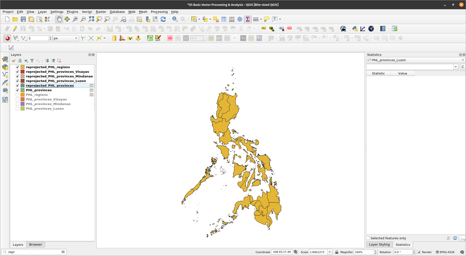
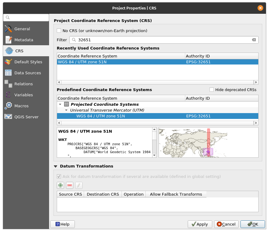
BONUS: Change the project CRS by clicking in the status bar found at the bottom right of the User Interface.

Change the project CRS to EPSG:32651.

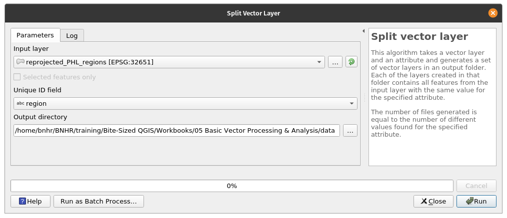
Splitting vectors

If we can merge vectors, it’s only natural that we can split vectors as well. For this exercise, let’s split the reprojected_PHL_regions layer into individual region layers.

Exercise 4: Splitting the regional polygon layer into individual region polygons

The Split vector layer algorithm takes a vector layer and an attribute and generates a set of vector layers in an output folder. Each of the layers created in that folder contains all features from the input layer with the same value for the specified attribute.

The number of files generated is equal to the number of different values found for the specified attribute.

NOTE: This algorithm respects the default vector format settings under the Processing toolbar. The file format of the output (split) files will use the default vector format.

1. Open the Split Vector Layer algorithm by searching in the Locator bar or via Vector -> Data Management Tools -> Split Vector Layer.

1. Input layer: reprojected_PHL_regions
2. Unique ID field: region
3. Output directory: your directory of choice

2. The output files can be found in the output directory provided.

Loading vectors from OSM

Exercise 5: Load a primary roads and schools from OSM

1. Filter the reprojected_PHL_provinces to show only the province of Albay.
2. Open the QuickOSM plugin and load primary roads using the following parameters:

1. Key: highways
2. Value: primary
3. Layer Extent: reprojected_PHL_provinces
4. Advanced:

1. Lines
2. Multilinestrings

3. Load schols using the following parameters:

1. Key: amenity
2. Value: school
3. Layer Extent: reprojected_PHL_provinces
4. Advanced:

1. Polygons

4. A highway_primary and amenity_schools layer should be added to the Layer Panel.
5. Reproject said layers to EPSG:32651 (Batch Process).
6. You should have a reprojected_highway_primary and reprojected_amenity_school layer with CRS equal to EPSG: 32651.

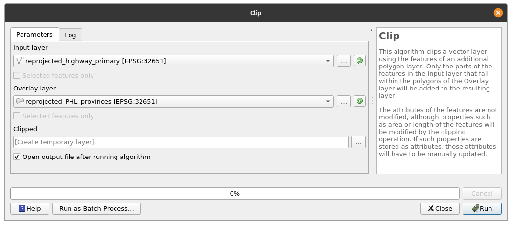
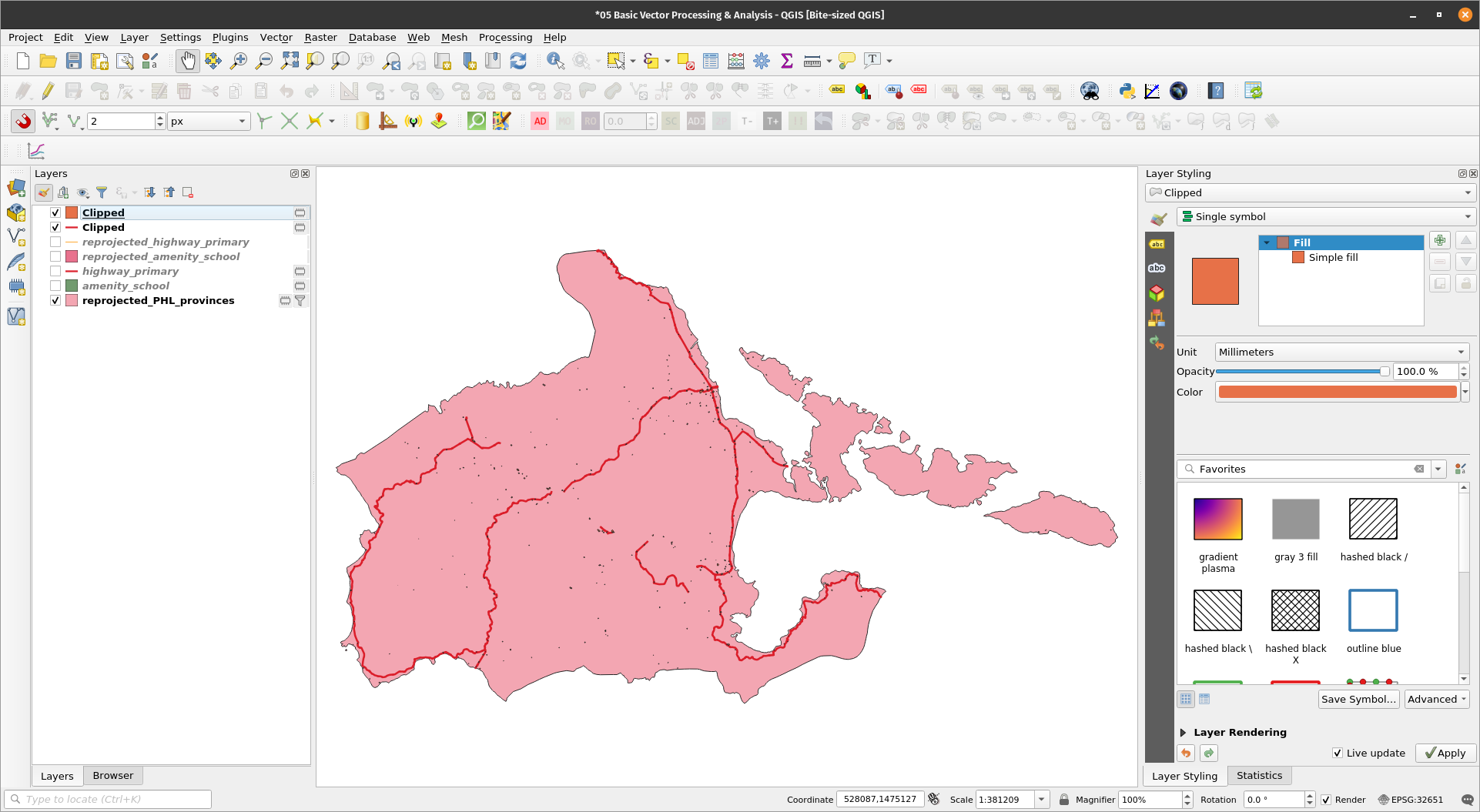
Clipping vectors

Notice that there are roads and schools located outside of the province of Albay. Since we only want the roads and schools inside the Albay feature, we can simply Clip the highway_primary and amenity_school layer with the reprojected_PHL_provinces layer.

Exercise 6: Clipping the primary roads and schools vector to the province of Albay

The Clip algorithm clips a vector layer using the features of another polygon layer. Only the parts of the features in the Input layer that fall within the polygons of the Overlay layer will be added to the resulting layer.

The attributes of the features are not modified, although properties such as area or length of the features will be modified by the clipping operation. If such properties are stored as attributes, those attributes will have to be manually updated

1. Open the Clip algorithm by searching in the Locator bar or via Vector -> Geoprocessing -> Clip in the Menu bar.

1. Input layer: reprojected_highway_primary
2. Overlay layer: reprojected_PHL_provinces

2. Click Run.
3. A new Clipped layer should appear in the Layer Panel.
4. Do the same for the reprojected_amenity_school layer (or do Batch Process).
5. You can renamed the Clipped layers to

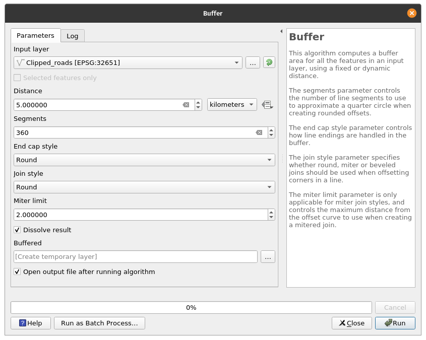
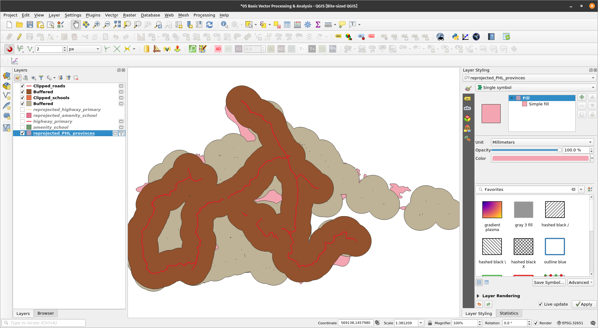
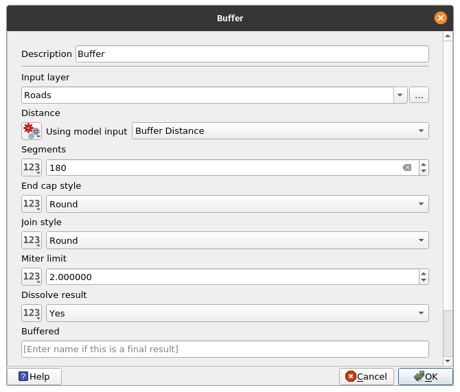
Creating buffers

Another common processing algorithm used are Buffers.  This algorithm computes a buffer area for all the features in an input layer, using a fixed or dynamic distance.

Buffers are an easy way to visualize nearness or inclusion of datasets. For example, we can try to find areas that are simultaneously within 5km of a road and 5km of a school by performing a buffer on the road and school layers and then running an intersection or clip algorithm on the resulting buffers.

Exercise 7: Creating a 5km buffer around the schools and road layers

1. Open the Buffer algorithm by searching in the Locator bar or via Vector -> Geoprocessing Tools -> Buffer in the Menu bar

2. Click Run.
3. Do the same for the Clipped_schools layer.
4. You should have 2 Buffered layers in the Layer Panel. You can rename these layers to Buffered_roads & Buffered_schools.

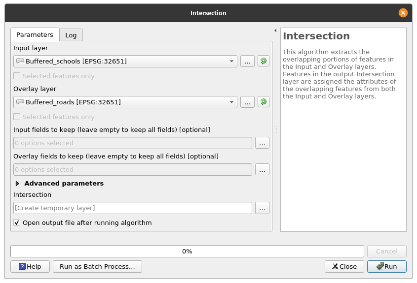
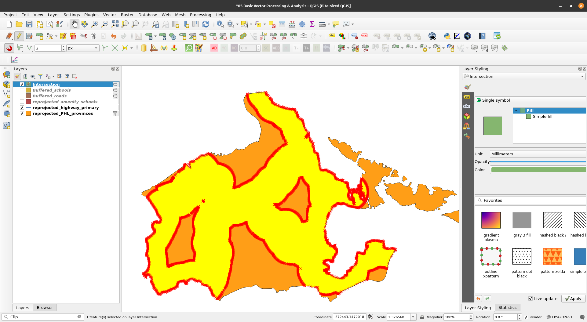
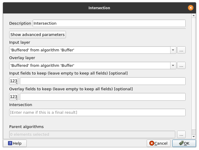
Intersecting vector layers

Now that we know the areas that are 5km from each school and 5km from the roads. We can now find areas that are simultaneously within those two buffers by using the Intersection algorithm.

BONUS: When to use Clip and when to use Intersection? Use a clip if you are only interested in the attributes of the base layer. Use Intersection if you want your output to have the attributes of the base layer and intersection layer.

Exercise 8: Find areas within 5km of a POI and a road.

The Intersection algorithm extracts the overlapping portions of features in the Input and Overlay layers. Features in the output Intersection layer are assigned the attributes of the overlapping features from both the Input and Overlay layers.

1. Open the Intersection algorithm from the Locator bar or via Vector -> Geoprocessing tools -> Intersection in the Menu bar.

1. Input layer: Buffered_schools
2. Overlay layer: Buffered_roads

2. Click Run

3. There should be a layer named Intersection in the Layer panel.

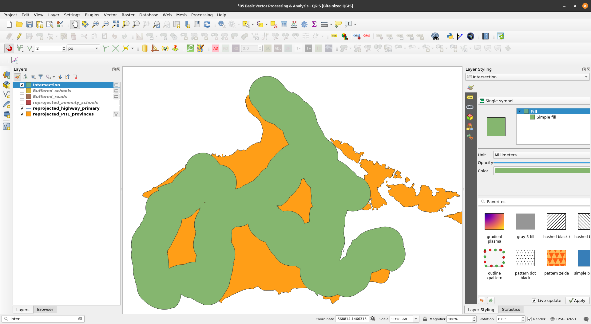
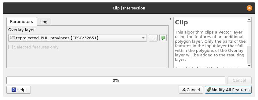
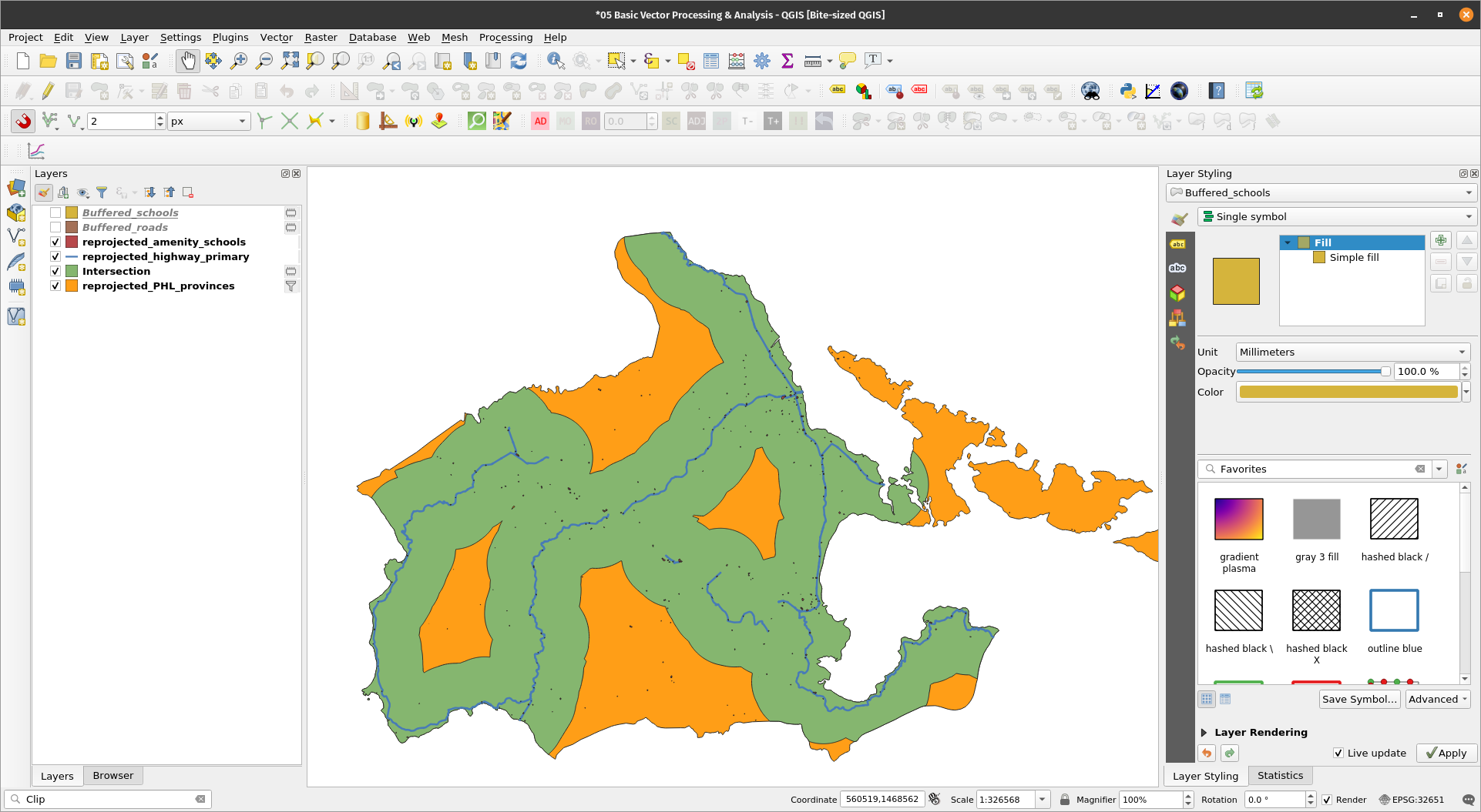
BONUS: Notice that there are areas that go beyond the boundaries of the province? What if I want to include only the areas within the province? We can perform another Intersection between the Intersection layer and the reprojected_PHL_provinces layer.

For certain vector algorithms, QGIS allows for in-place editing. This means that the algorithm will not create a new output but edit the input layer instead.

1. Make sure that the Intersection layer is selected/active.
2. Search for Clip in the Locator bar and select the one under Edit Selected Features.

3. The Intersection layer should now be edited. Make sure to save the edit by clicking  in the Digitizing toolbar.

These are now the areas within Albay that are both within 5km of a primary road and a school.

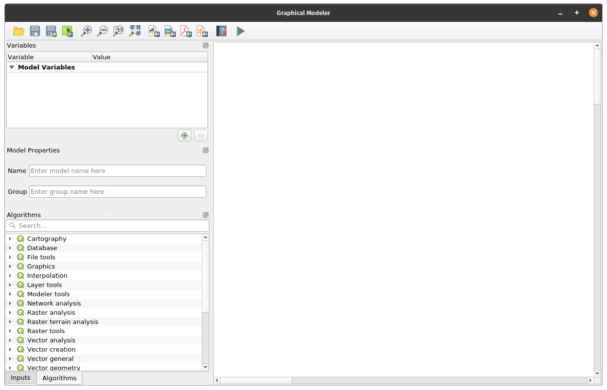
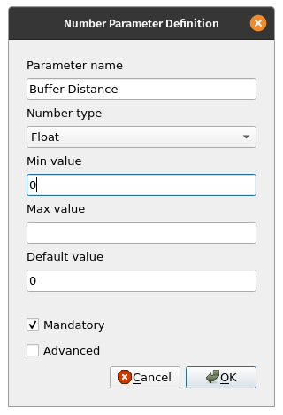
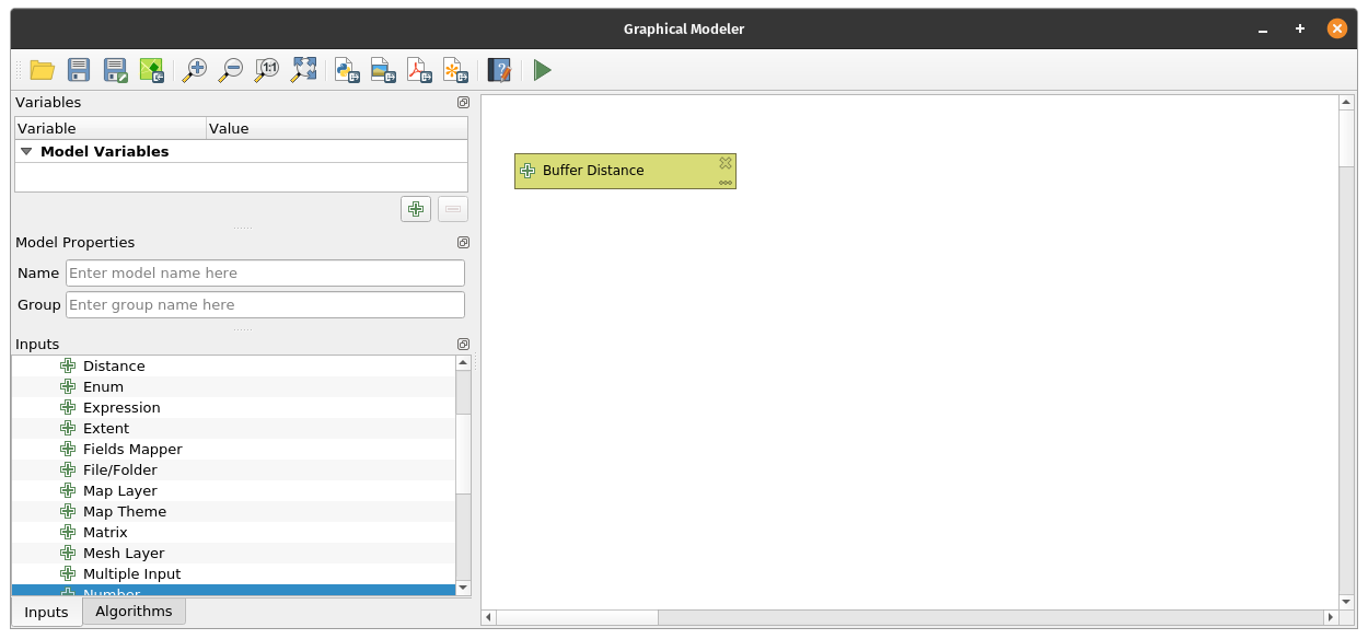
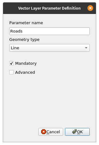
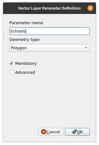
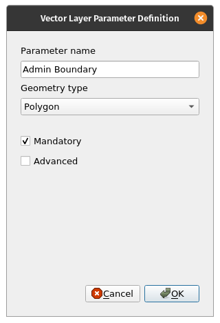
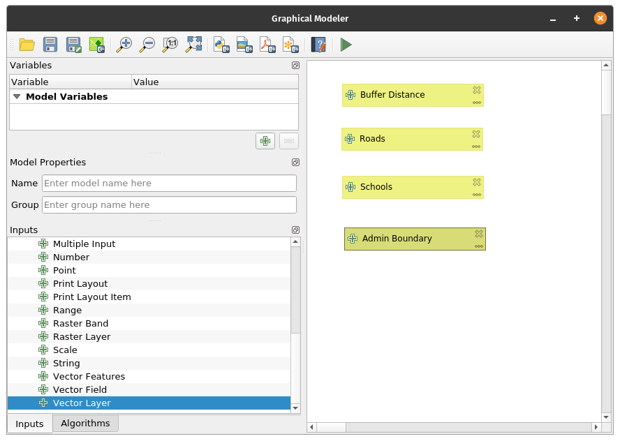
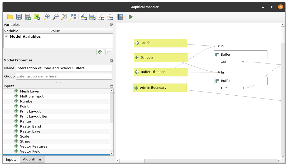
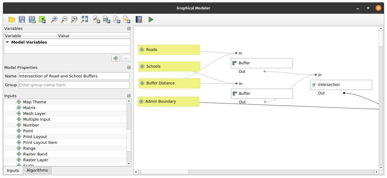
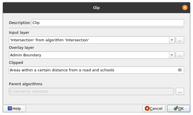
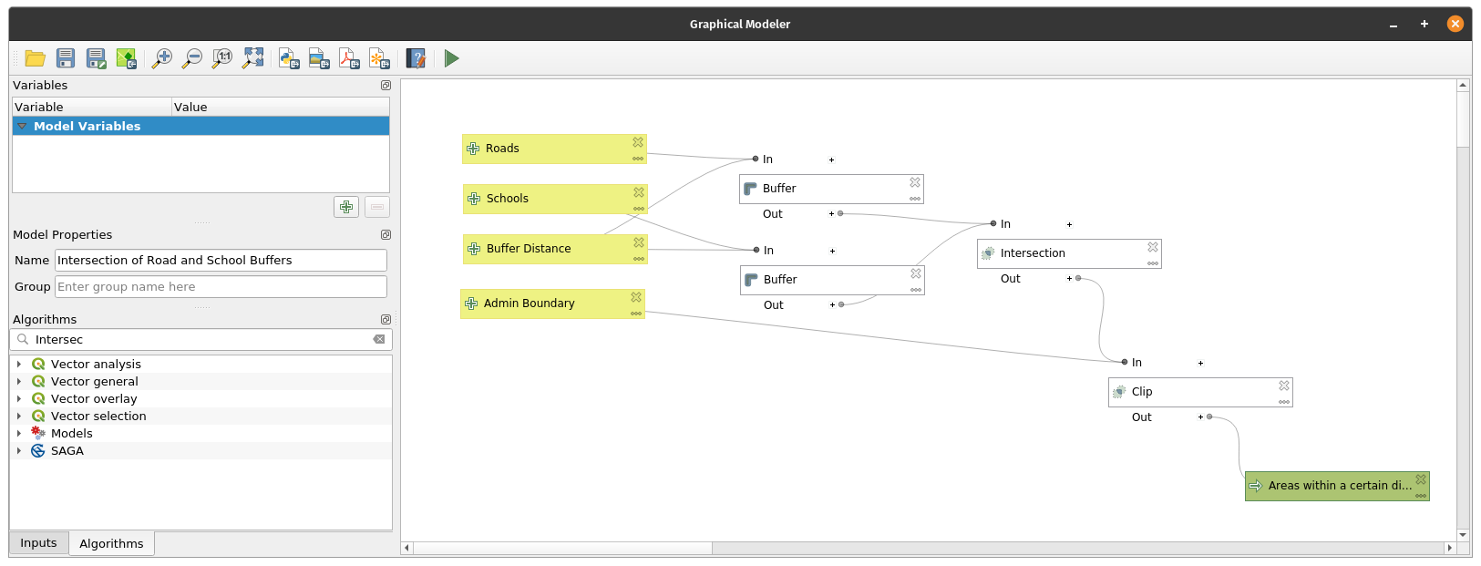
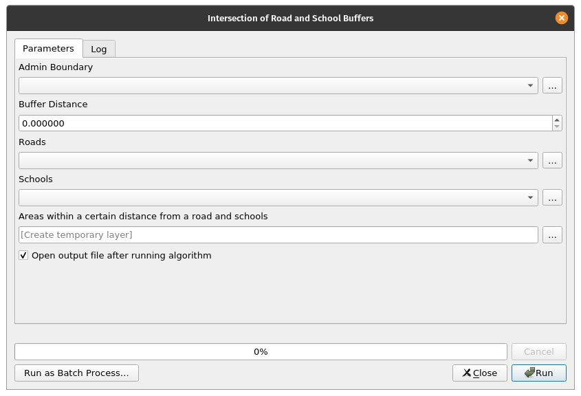
QGIS has a powerful graphical modeler that allows you to create reusable and shareable models. These models can also be converted into Python scripts easily.

One of the advantages of using models is that we can easily change inputs and variables without needing to run the algorithms multiple times. For example, let’s create a simple model of our process for getting the areas within a province that are a certain area from roads and schools.

Exercise 9: Creating a simple model with the graphical modeler

1. Open the Graphical Modeler via Processing -> Graphical Modeler.
2. This will open the Graphical Modeler window. On the right is the model canvas where we can drag-and-drop Inputs and Algorithms from the left side.

3. First let’s add a Number Input to our model. This will hold the Buffer Distance value.

4. Then we add three Vector Layer Inputs to our model -- one for the Roads (line), Schools (polygon), and Admin Boundary (polygon).

5. Then we add the 2 Buffer Algorithms (1 for Roads and 1 for Schools). Use a model input (Buffer Distance) fro the Distance parameter.

6. Afterwards, we add an Intersection Algorithm to intersect the results of our Road and Schools buffer.

7. Lastly, add a Clip Algorithm to clip the result of the intersection and the Admin Boundary layer.

8. You can save this model by using . Saved models can be accessed under Models in the Processing Panel.
9. You can run the model with . Upon running the model, it will ask us to provide inputs.

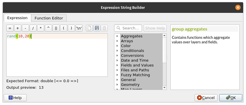
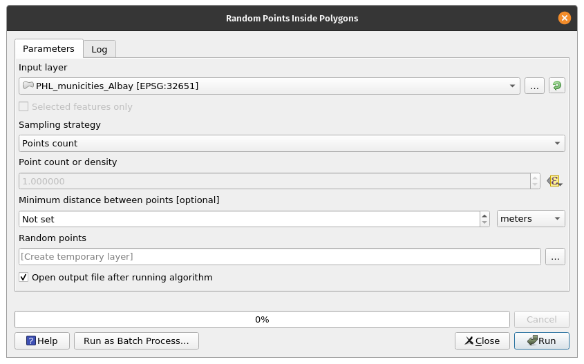
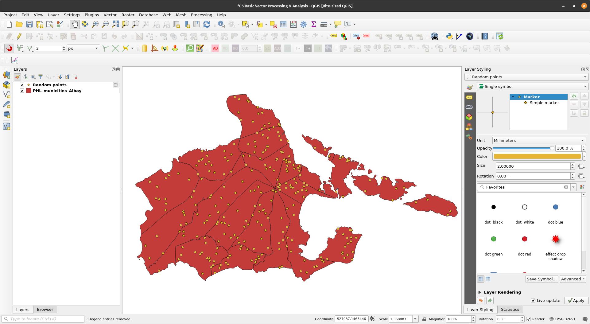
Generating random points inside polygons

Exercise 10: Generate random points inside the PHL_municities_Albay layer

The Random Points Inside Polygon algorithm allows users to generate random points inside polygons. The number of points can be set by a point count or point density value. This value, as with other algorithm parameters, can be defined by a data-defined override.

1. Open the Random Points Inside Polygons algorithm by searching in the Locator bar or via Vector -> Research Tools -> Random Points Inside Polygons.

1. Input layer: PHL_municities_Albay
2. Sampling strategy: Points count
3. Point count or density: Data-defined override

2. Click Run.
3. A Random Points layer should be added to the Layer Panel.

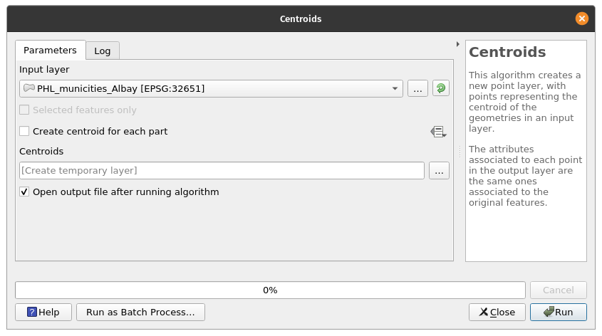
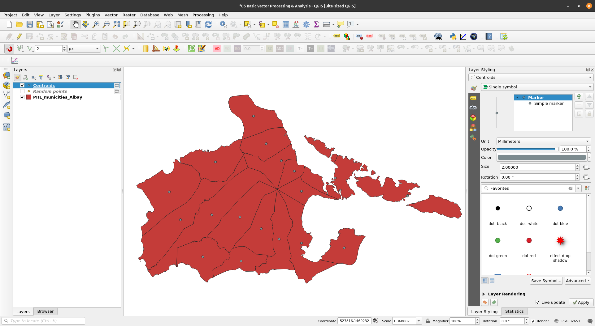
Getting centroids

Exercise 11: Create a centroid layer of the PHL_municities_Albay layer

The Centroids algorithm creates a new point layer, with points representing the centroid of the geometries in an input layer. The attributes associated with each point in the output layer are the same ones associated with the original features.

1. Open the Centroid algorithm by searching in the Locator bar or via Vector -> Geometry Tools -> Centroids..

1. Input layer: PHL_municities_Albay

2. Click Run.
3. A new Centroids layer should be added to the Layer Panel.

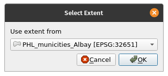
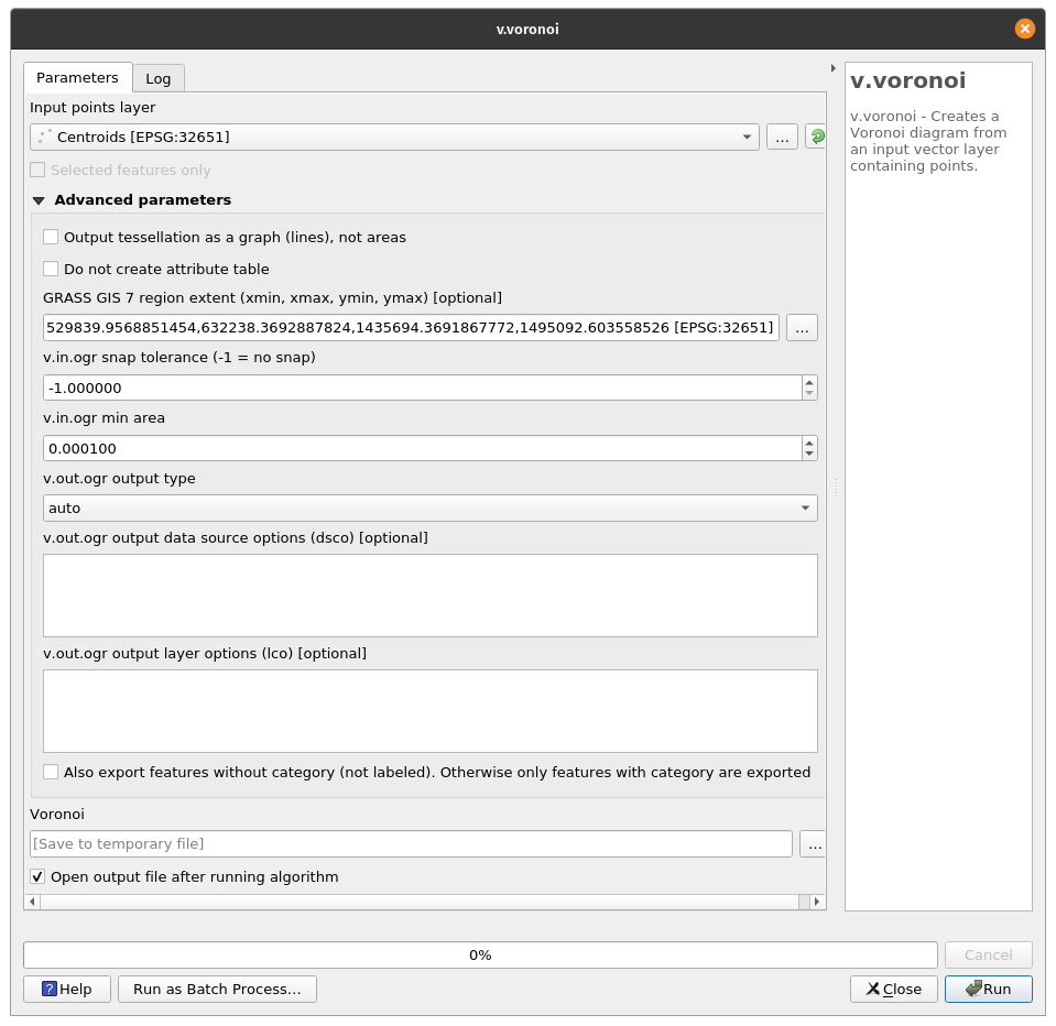
Find the points from one layer that are nearest to each point from another layer

Exercise 12: Voronoi polygons

Aside from QGIS processing algorithms, QGIS also has access to algorithms from processing providers connected to it. These include GRASS, SAGA, Orfeo Toolbox, TauDEM, LASTools, etc.

For this exercise, we’ll use the v.voronoi algorithm from GRASS GIS to generate voronoi polygons from the Centroids we generated earlier.

Voronoi polygons are generated from points. If a point is inside a voronoi polygon, it means that it is nearest to the generating point of that polygon than all generating points.

A possible use case of voronoi or Thiessen polygons is finding the closest cell tower to a user given the location of cell towers.

For our exercise, we can use voronoi polygons to determine the random points that are closest to our city/municipality centroids.

1. Open the v.voronoi algorithm from the Locator bar or under GRASS -> Vector -> v.voronoi in the Processing Panel.

1. Input points layer: Centroids
2. Advanced parameters:

1. GRASS GIS7 Region: Use Layer Extent of PHL_municities_Albay. Click  -> Select Layer Extent...

2. Click Run.
3. A Voronoi layer should be added in the Layer Panel.

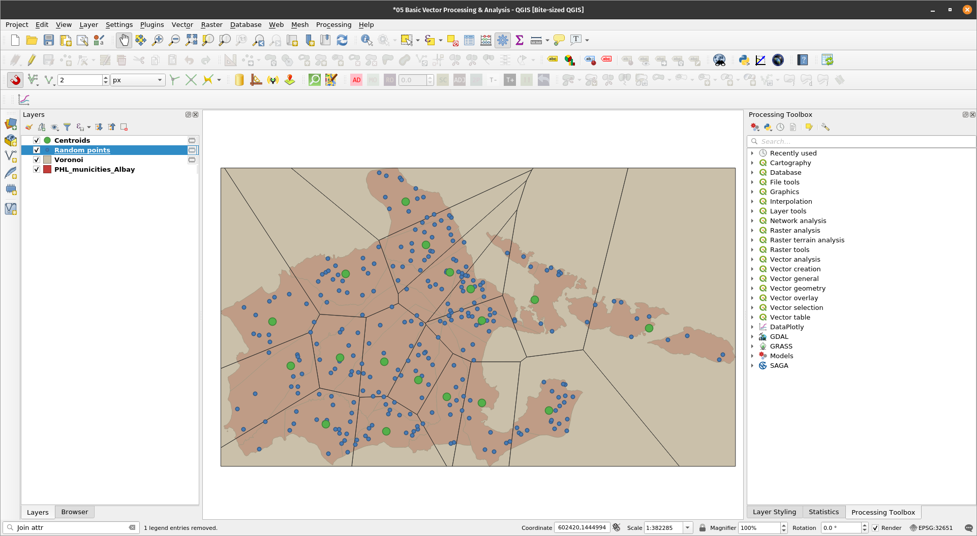
The resulting Voronoi layer contains the same attributes as the input point layer (Centroids). We can then use the join attributes by location on the Random Points and Voronoi layer to determine which City/Municipality centroid the point in the former is closest to.

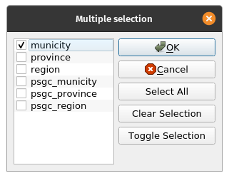
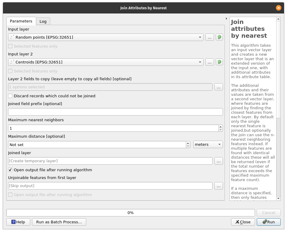
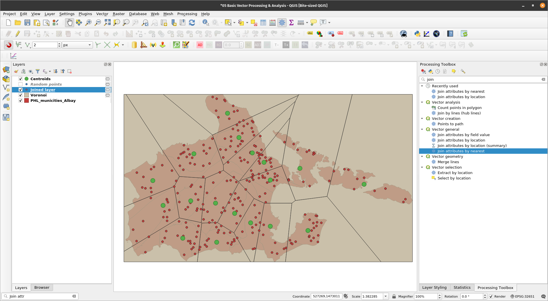
Exercise 13: Join attributes by nearest

QGIS also has a built-in algorithm to Join attributes by nearest. This algorithm takes an input vector layer and creates a new vector layer that is an extended version of the input one, with additional attributes in its attribute table.

The additional attributes and their values are taken from a second vector layer, where features are joined by finding the closest features from each layer. By default only the single nearest feature is joined,but optionally the join can use the n-nearest neighboring features instead. If multiple features are found with identical distances these will all be returned (even if the total number of features exceeds the specified maximum feature count).

1. Open the Join attributes by nearest algorithm from the Locator bar or under Vector general -> Join attributes by nearest in the Processing Panel.

1. Input layer: Random points
2. Input layer 2: Centroids
3. Layer 2 fields to copy: municity

2. Click Run.
3. A Joined layer layer should be added in the Layer Panel.

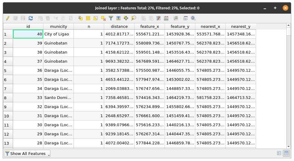
The attributes of this Joined layer includes the attributes from the Input layer (Random points), the attribute copied from Input layer 2 (Centroids), new attributes for the distance to the near features (distance), the index of the feature (n), and the coordinates of the closest point on the input feature (feature_x, feature_y) to the matched nearest feature, and the coordinates of the closet point on the matched feature (nearest_x, nearest_y).

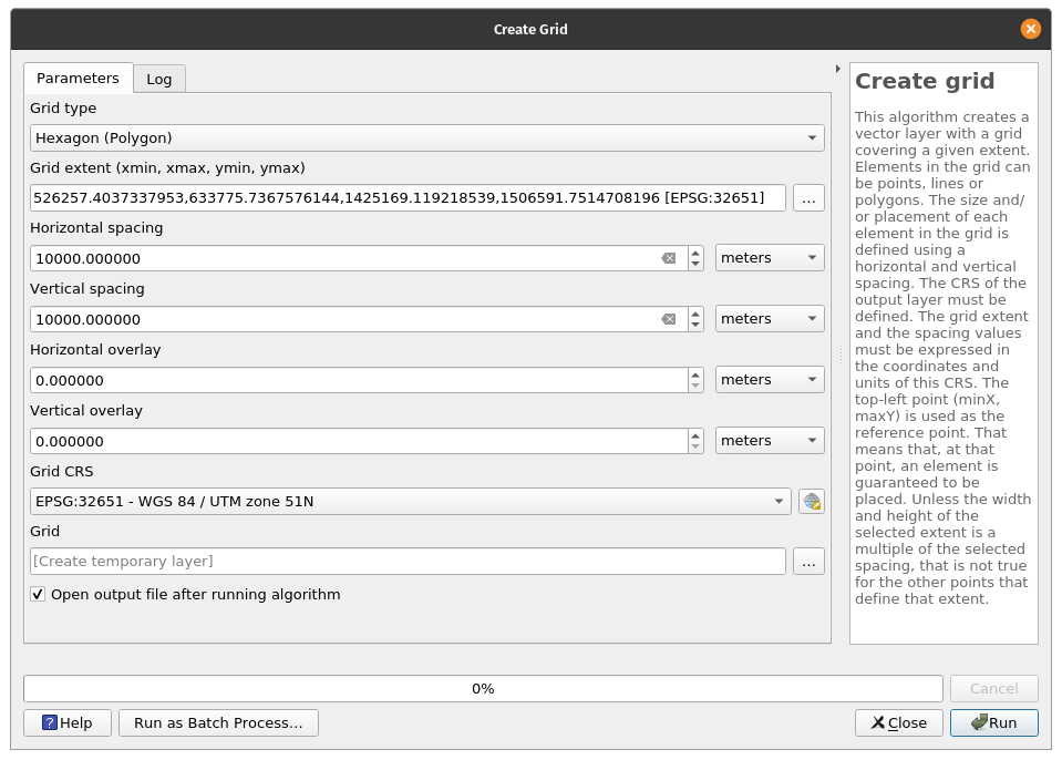
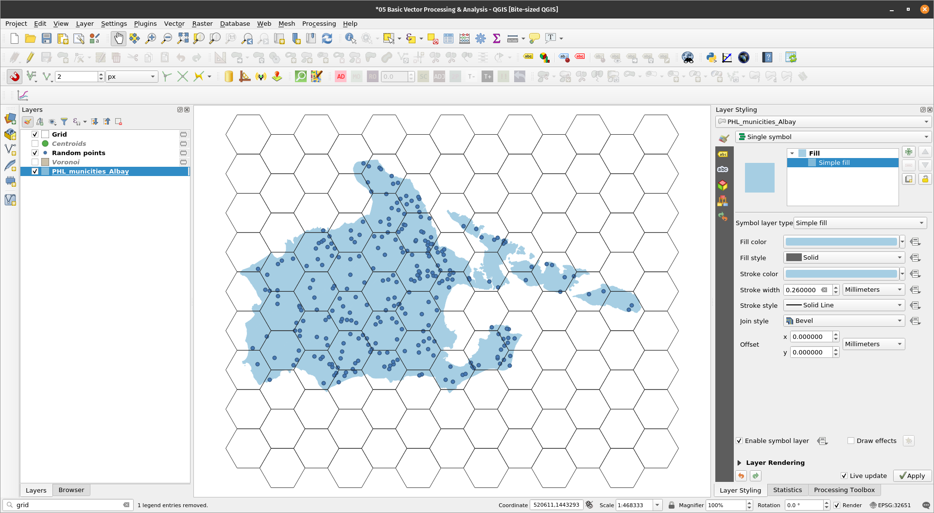
Creating grids

Exercise 14: Generating grids in QGIS

QGIS also has an algorithm to generate grids. These grids can be made up of points, squares, diamonds, or hexagons. In this exercise, let’s create a hex grid -- a very common and popular means of visualizing data.

1. Right-click PHL_municities_Albay -> Zoom to layer.
2. Open the Create grid algorithm from the Locator bar or via Vector creation -> Create grid in the Processing Panel.

1. Grid type: Hexagon (Polygon)
2. Grid extent: use Canvas extent
3. Horizontal spacing: 10000 m
4. Vertical spacing: 10000 m

3. Click Run.
4. A new Grid layer should be added in the Layer Panel.

You can then use this grid for other processing and analysis (e.g. zonal statistics, counting points in polygon, summarizing per grid, etc.)

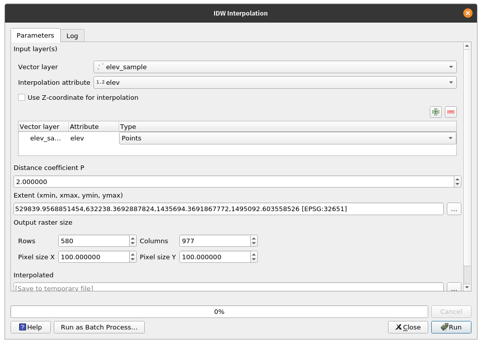
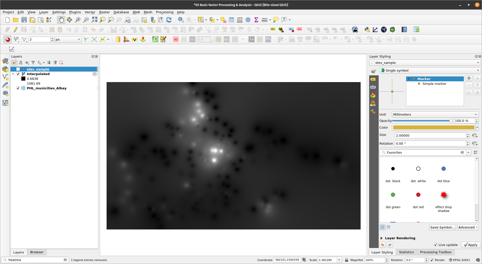
There are several interpolation methods available to QGIS -- IDW, Regularized Spline with Tension, etc. These are available as core QGIS processing algorithms or via GRASS, SAGA, and other external processing providers.

Exercise 15: IDW Interpolation

1. Load the elev_sample point layer.
2. Open the IDW interpolation algorithm from the Locator bar or under Interpolation -> IDW interpolation in the Processing Panel.

1. Input layer(s):

1. Vector layer: elev_sample
2. Interpolation attribute: elev

2. Extent: Use Layer extent (elev_sample)
3. Pixel size: 100

3. Click Run.
4. A new Interpolated layer should appear in the Layer Panel.

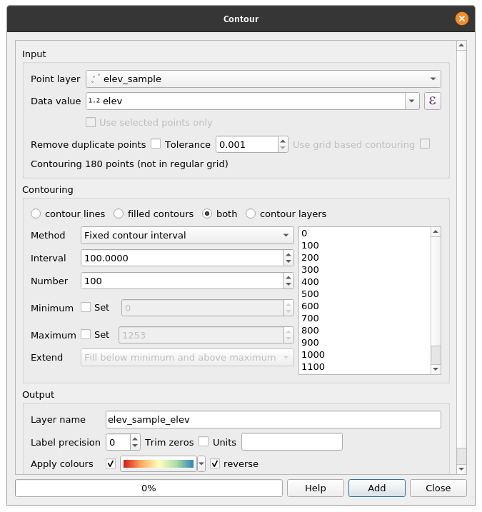
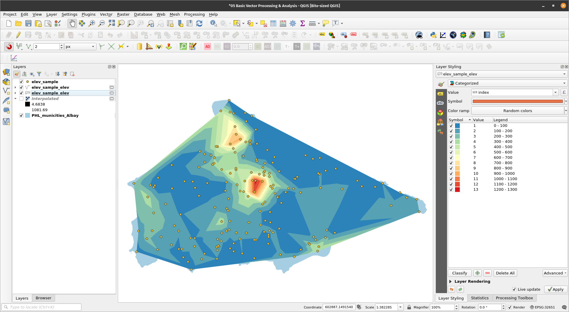
Exercise 16: Contours from points

Contours can be generated from a set of points by using the Contour plugin .

1. Open the Contour plugin.

1. Point layer: elev_sample
2. Data value: elev
3. Contouring:

1. Both
2. Method: Fixed Contour Interval
3. Interval: 100
4. Layer name: elev_sample_elev

2. Click Run.
3. There should be an elev_sample_elev line and polygon layer in the Layer Panel.

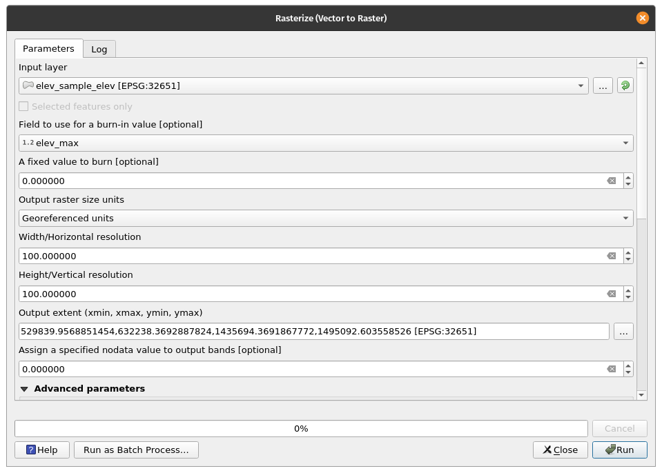
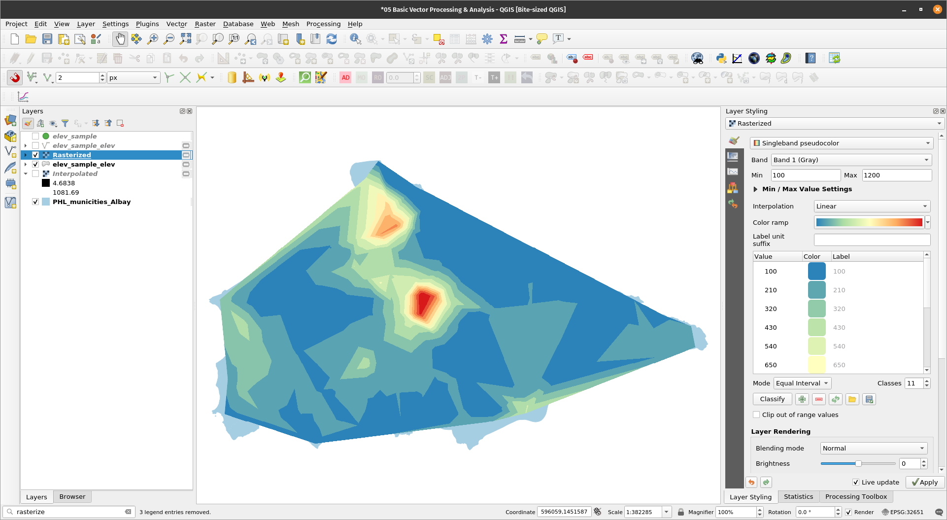
Sometimes we need to convert vectors to rasters and vice versa.

Exercise 17: Converting the contour polygon to a raster

1. Open the Rasterize (vector to raster) algorithm from the Locator bar, via Raster -> Conversion -> Rasterize (Vector to Raster) in the Menu bar, or under GDAL -> Vector conversion -> Rasterize (vector to raster) in the Processing Panel.

1. Input layer: elev_sample_elev
2. Field to use: elev_max
3. Output raster size units: Georeferenced units
4. Resolution: 100
5. Output extent: Use Layer Extent (PHL_municities_Albay)

2. Click Run.
3. A Rasterized layer should be added to the Layer Panel.